
Process simulation and optimization with the help of numerical methods can reduce expensive and time consuming experiments for manufacturing good quality products. Electroplating is a prominent coating process that the quality and uniformity of the deposition are of great importance in this process. In this paper a finite element model has been proposed for evaluation of primary and secondary current density values on the cathode surface in nickel electroplating operation of a revolving part. In addition, the capability of presented electroplating simulation has been investigated in order to describe the electroplated thickness of the nickel sulfate solution. Nickel electroplating experiments have been carried out and the measured thickness in different points have been compared with the predictions. A good agreement between the simulated and experimental results was found. Also the results showed that primary current density can describe the general form of thickness distribution but the relative value of current density using secondary current density can present better description of thickness distribution.
Introduction
The importance of electro deposition as a coating technology is large and growing in different field industry. With the current behavior in the cost competitive products, electro deposition is one of the important manufacturing process that still remain strongly [1].
In all electro deposition applications, thickness uniformity is one of the most important characteristics. So many different techniques were established for achieving uniform thickness. During the years, researchers in the field of electroplating and electroforming always tried to predict the thickness of coatings deposited on the parts or mandrels. Mathematical modeling has been used to describe the electroplating process. One of the fist models was introduced by McGeough and Rasmussent [2]. They used perturbation analysis to find a model to achieve more uniform thickness distribution on a mandrel surface with sinusoidal mandrel surface with irregularities. Also they analyzed electroforming process with direct current by perturbation method [3, 4]. The mathematical model was limited to simple model shapes of cathode and anode. By using numerical methods such as finite element analysis (FEA) one can simulate more complex shapes and conditions compared to analytical modeling. Many researchers have been used FEA for electroplating process simulation. Yang et al. [5] simulated primary current density of nickel electroplating process and compared its values with relative thickness. Also Zhu et al. [6] applied primary current density FE simulation on the cathode surface of near-polished surface of nickel. They showed that the simulated current density curve is similar to relative thickness curve. Masuku et al. [7] used 2D and 3D finite element analysis to determine the local plating depth for copper plating process. They found that 3D model has a good agreement with profile of the real plated surface. In this research after conducting electroplating experiments, the coating thickness of different points was measured. Primary and secondary current density was simulated using the commercial FE software code COMSOL and the relative value of thickness and current density compared with each other.
Electroplating theory
In electroplating process, the deposited thickness distribution and other properties like surface texture and morphology are directly related to current distribution. Current distribution can be analyzed in two different macro and micro scale. Macroscopic scale is about solving models on the order of centimeter and is to analyze thickness distribution. Micro scale is about sub millimeter length scale and is to analyze deposit texture and roughness, nucleation.
Based on Faraday’s law in electrochemistry, if we find the current density value on different points on cathode surface, we can predict the deposited metal layer. In this paper the macroscopic current density distribution was studied. There are some simplifying approximations for electroplating simulation. Primary, secondary, mass transport and tertiary current density are common approximations for modeling the current distribution. Because in this article we study the primary and secondary current density distribution for nickel electroplating process, so in following sub sections we introduce these two kinds of approximations.
Primary Current Density
Based on Newman theory, the potential V obeys Laplace equation in the electrolyte.
![]()
In the boundary condition at all insulating boundary or symmetry plane is
![]()
Where n is a unit vector normal to the surface. In this kind of approximation just Ohmic irregularities were considered kinetic and mass transport limitations were neglected.
Secondary Distribution
If we considered both, Ohmic and Kinetic irreversibility, the simulated current called secondary current density. In this kind of approximation the mass transport limitation was neglected.
In this condition Laplace equation will solve with following boundary condition
Insulator:
![]()
Cathode surface:
![]()
Where ηs and i is related to each other by Tafel equation
![]()
Where Ac is the slope of Tafel line. iloc is local current density , io exchange current density.
Experimental Procedure
Figure 1 shows a schematic diagram of the electroplating system used in this research. This system has a rolled rounded nickel anode and cylindrical aluminum mandrel.
![Fig. 1: A sketch of electroforming System [8].](https://www.jept.de/wp-content/uploads/2015/05/electroplatingbild1.png)
Fig. 1: A sketch of electroforming System [8].
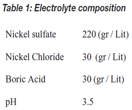
The nickel sulfate solution was used as the electrolyte. Its composition is shown in Table 1.
Aluminum mandrel with a complex cylindrical shape was degreased with organic solvent and rinsed. After plating process The sample was cut from its central axis with WEDM (Wire Electro Discharge Machining). Sample was mounted polished and thickness was measured using optical microscope.
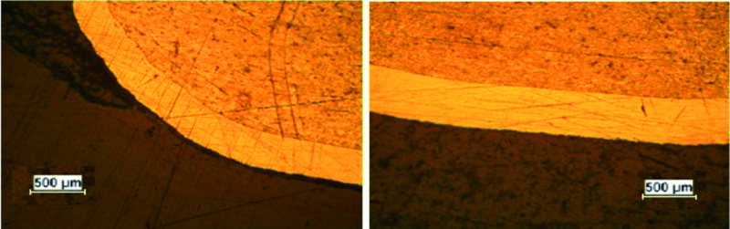
Fig. 2: Electroplated sample
Finite Element Model
The Finite Element Method (FEM) is a numerical method for solving differential and integral equations. In this method, the unknown variables to be determined are approximated by piecewise continuous functions. The coefficients of the functions are adjusted in such a manner that the error in the solution is minimized. Usually, the coefficients of the functions of a particular element are the values at certain points in the element called nodes. During the solution process, the differential equations get converted to algebraic equations or ordinary differential equations that can be solved by finite difference equations. The finite element method consists of the following steps: (I) Pre-processing; (II) Developing elemental equations; (III) Assembling equation; (IV) Applying boundary conditions; (V) Solving the system of equations; and (VI) Post-processing. A FE numerical model was developed for electroplating simulation. A 2D geometric model of anode and cathode surface and also electrolyte was constructed. Defined geometry for finite element simulation is shown in Figure 3. Geometry was defined by key points, lines and curves to define an area that electroplating process happens in it.

Fig. 3: Defined geometry for finite element simulation
To define cathode, anode and electrolyte a value of electrical conductivity and electrical voltage was applied. Also for simulating secondary current density, surface kinetic was applied to the cathode surface using Tafel equation. After conducting preprocess phase of FE model, the defined finite element model passed for the solution. Applied 2D elements for simulation is shown in Figure 4.
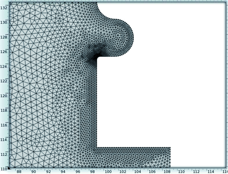
Fig. 4: Applied 2 dimensional elements for simulation
During the FE solution, solver yields the potential and current density on each node. The value of primary and secondary current density was extracted in the points that their thickness was measured before. Figure 5 shows the simulated current density in electrolyte. 3D graph of simulated current density is illustrated in Figure 6.
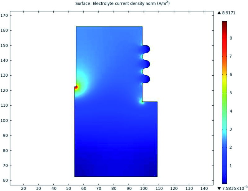
Fig. 5: Simulated Current Density in electrolyte
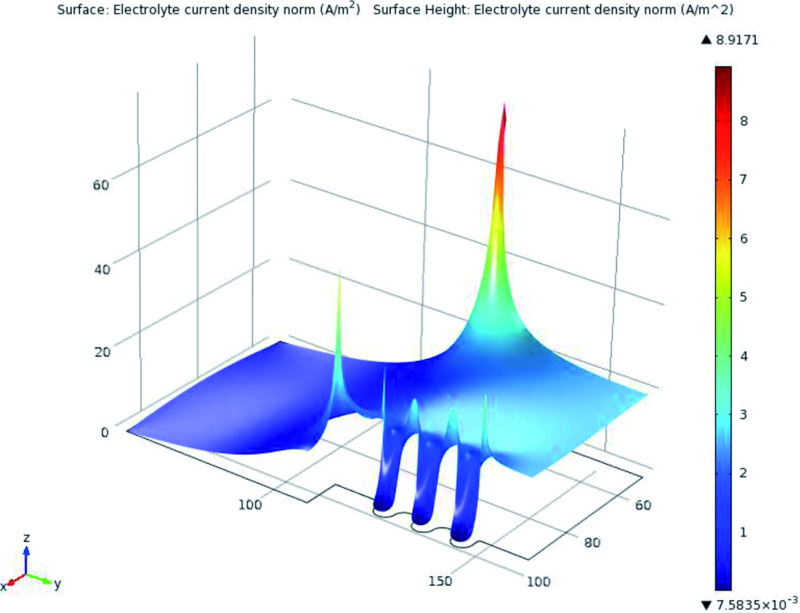
Fig. 6: 3 Dimensional Graph of simulated current Density
Comparison of Results
In Figure 7, the relative value of thickness is compared with relative value of primary and secondary current density. Relative value is defined as follow.
![]()
Where n is the number of measured value, tk is the value (thickness or current density) at the selected position.
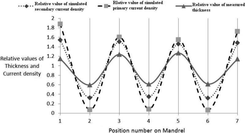
Fig. 7: Comparison of results
According to Figure 7, all three curves show the same profile trend. At the points with higher diameter more thickness was deposited and also in comparison with other points, the simulated primary and secondary current density have higher relative value. However the actual divergence between measured thickness and simulated current density, at the edge of mandrel is increased compared with other points.
Also it can be described that relative value of simulated secondary current density has a better agreement with relative thickness value compared with relative value of simulated primary current density. After applying surface kinetic boundary condition by use of Tafel equation, maximum value of simulated primary current density was decreased and minimum value was increased. It shows that the primary current density has a major effect on thickness distribution in nickel electroplating process, but by applying surface kinetic limitation on finite element model, the thickness distribution can be described with more precision.
Conclusion
An experimentally supported 2D finite element simulation of the nickel electroplating process was presented in this paper. The relative values of thickness, primary and secondary current density, obtained from simulation, were compared to those of experiments. It was seen that simulation data is in good agreement with experiments. Also it was shown that the secondary current density distribution has a better agreement with relative thickness distribution in nickel electroplating with nickel sulfate solution.
References
- J. O. Dukovic, “Computation of current distribution in electrodeposition, a review,” IBM Journal of Research and Development, 34 (1990) 693.
- H. R. J.A.McGeough, „Aperturbation Analysis Of Electroforming Process,“ Journal of Mechanical Engineering Science, 18 (1976).
- H. R. J.A.McGeough, „Theorical Analysis of the electroforming process,“ journal of Mechanical Engineering Science, vol. 23 (1981) 113.
- H. R. J.A.McGeough, „Analysis of electroforming with direct current,“ Journal of Mechanical Engineering Science, vol. 19 (1977) 163.
- J.-M. Yang, D.-H. Kim, D. Zhu, and K. Wang, „Improvement of deposition uniformity in alloy electroforming for revolving parts,“ International Journal of Machine Tools and Manufacture, vol. 48 (2008) 329.
- Z. W. Zhu, D. Zhu, N.-S. Qu, K. Wang, and J.-M. Yang, „Electroforming of revolving parts with near-polished surface and uniform thickness,“ International Journal of Advanced Manufacturing Technology, 39 (2008) 1164.
- E. S. Masuku, A. R. Mileham, H. Hardisty, A. N. Bramley, C. Johal, and P. Detassis, „A Finite Element Simulation of the Electroplating Process,“ CIRP Annals – Manufacturing Technology, vol. 51 (2002) 169.
- A. M. Behagh, A. R. Fadaei Tehrani, H. R. Salimi Jazi, and S. Zare Chavoshi, „Investigation and optimization of pulsed electroforming process parameters for thickness distribution of a revolving nickel part,“ Proceedings of the Institution of Mechanical Engineers, Part C: Journal of Mechanical Engineering Science, doi: 10.1177/0954406212473409
PDF Version of the article |
Flash Version of the article |
|
| [qr-code size=”2″] | ||